SDF Path Tracing 2
Addison Prairie / August 23
Recently, while on a plane ride, I decided to write a small signed distance function (SDF) path tracer to learn some new techniques. This article will probably be fairly short since I did not do too much on this (mini) project; however, I still wanted to go over some of the things I learned and show some interesting renders. Clicking on each of the images below will open a demo page which renders them live (NOTE: each requires WebGPU).
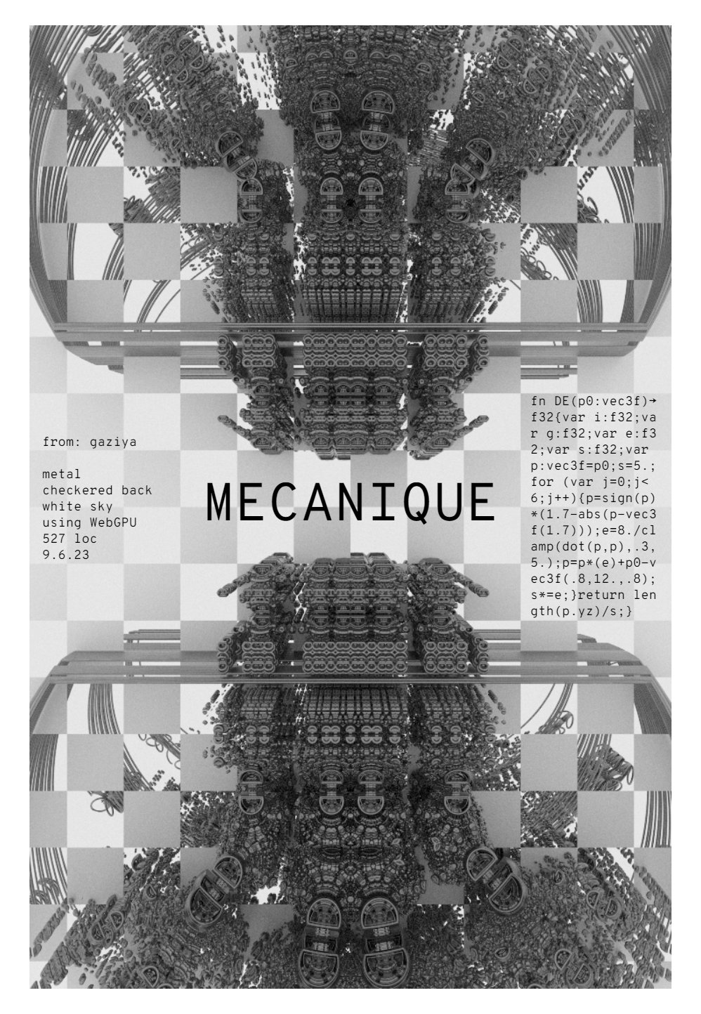
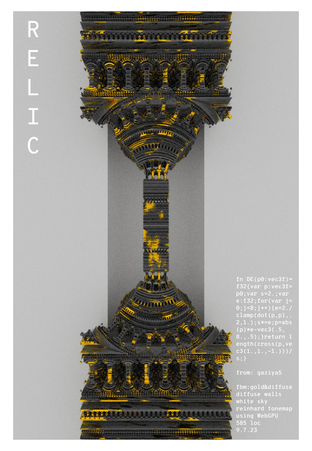
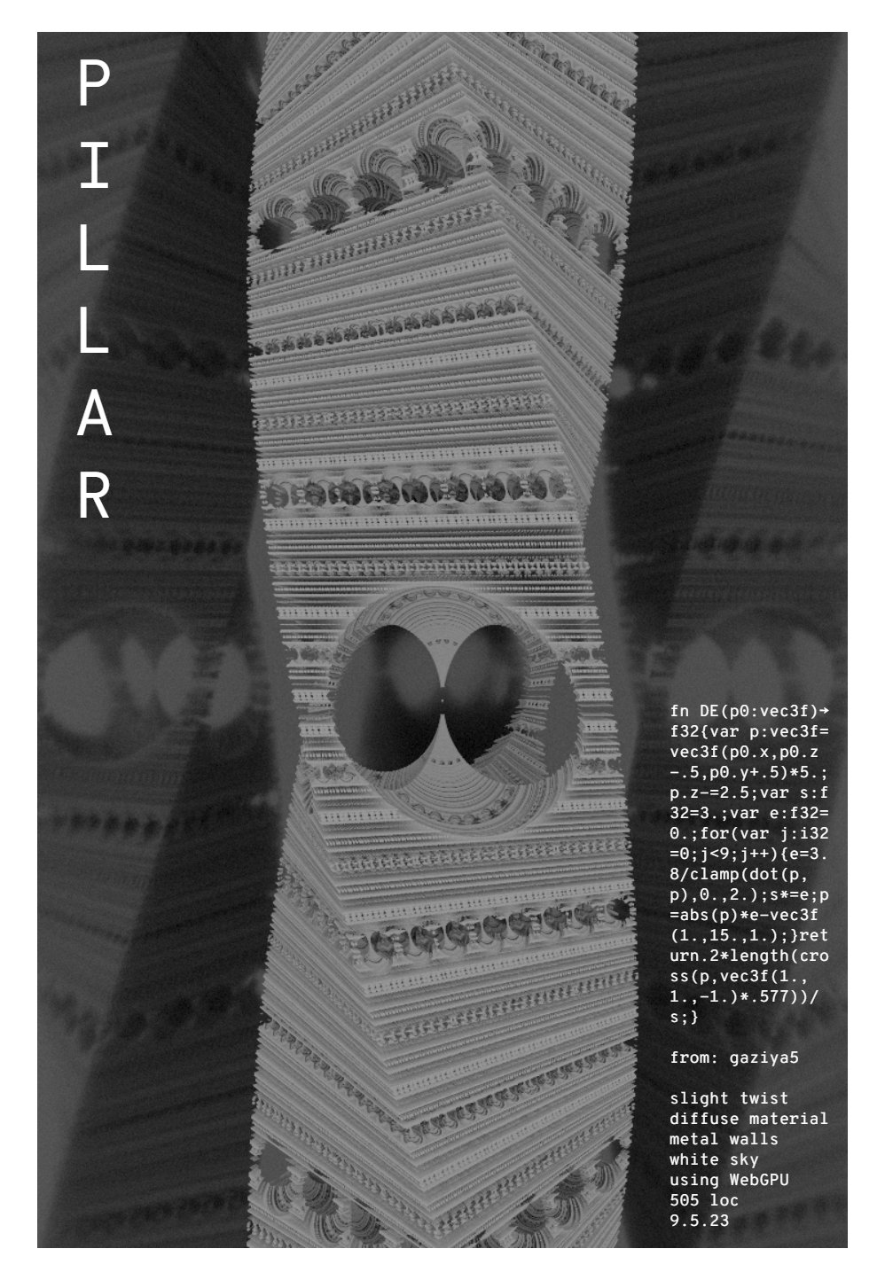
Three path traced SDFs using procedural solid texturing and GGX-Smith microfacet model for rough specular reflections.
1. GPU SDF Path Tracing
One of the things I wanted to learn more about for this project was path tracing scattering media, like clouds, smoke, and skin. However, media which have a high probability of scattering light are difficult to path trace on the GPU because a ray which enters them may require many iterations to terminate; as described briefly in my writing about wavefront path tracing, a port of the standard CPU path tracing loop will suffer greatly from thread divergence, especially when a large number of iterations are required for a ray to terminate. Thus, a different model of path tracing must be used. In my article, I gave the following code snippet of a path tracing loop which regenerates rays each iteration to decrease the number of idle threads in a workgroup:
1
2
3
4
5
6
7
8
9
10
11
12
13
14
15
16
17
18
19
20
21
22
23
24
25
26
27
28
29
30
2
3
4
5
6
7
8
9
10
11
12
13
14
15
16
17
18
19
20
21
22
23
24
25
26
27
28
29
30
//assuming position o, direction d are already defined

//t is the light accumulated across the path
var t = vec3f(0.);
var b = vec3f(1.);

var samples = 0;

for (var i = 0; i < MAX_BOUNCES; i++) {
    var normal : vec3f;
    var   dist :   f32;

    var bHit : bool = trace(o, d, &normal, &dist);

    //if path did not hit an object, accumulate sky color and break
    if (!bHit) {
        t += b * SKY_COLOR;
        samples++;

        regenerateCameraRay(&o, &d);
        b = vec3f(1.);
    } else {
        o = o + d * dist + normal * .001;

        b *= Sample_f_lambert(normal, &d);
    }
}

//safeguard to prevent NaN
var sumColor = samples == 0 ? vec3f(0.) : t / f32(samples);
For this project, I ended up using a very similar style of loop. The entire path tracer fits into a single GPU kernel, making it easy to debug. For each pixel in the image, 4 things are stored in memory: the path position (o), the path direction (d), the path throughput (b), and the pixel's accumulated samples (t). The shader is structured like this:
1
2
3
4
5
6
7
8
9
10
11
12
13
14
15
16
17
18
19
20
21
22
23
24
25
26
27
28
29
30
31
32
2
3
4
5
6
7
8
9
10
11
12
13
14
15
16
17
18
19
20
21
22
23
24
25
26
27
28
29
30
31
32
//[o.x, o.y, o.z, random_seed]
@group(0) @binding(0) var><storage, read_write> oBuffer : array<vec4f>;
//[d.x, d.y, d.z, num_bounces]
@group(0) @binding(1) var><storage, read_write> dBuffer : array<vec4f>;
//[b.x, b.y, b.z, ~]
@group(0) @binding(0) var><storage, read_write> bBuffer : array<vec4f>;
//stores accumulated samples
@group(0) @binding(0) var><storage, read_write> tBuffer : array<vec4f>;

@compute @workgroup_size(8, 8, 1)
fn main(@builtin(global_invocation_id) global_id : vec3u) {
    //check we don't have thread out of bounds
    if (outOfImageBounds(global_id.xy)) {return;}

    var bufferIndex = dot(global_id.xy, SCREEN_WIDTH);

    //fetch path state from memory
    var o = oBuffer[bufferIndex];
    var d = dBuffer[bufferIndex];
    var b = bBuffer[bufferIndex];
    var t = tBuffer[bufferIndex];

    for (var i = 0; i < ITER_PER_INVOCATION; i++) {
        extendPath(global_id.xy, &o, &d, &b, &t);
    }

    //send incremented path state to memory
    oBuffer[bufferIndex] = o;
    dBuffer[bufferIndex] = d;
    bBuffer[bufferIndex] = b;
    tBuffer[bufferIndex] = t;
}
Here are some notes about the parts of this code:
- Memory Alignment: because of the way GPUs are designed, a 12 byte vector (i.e., vec3f, vec3i, etc.) must be read from memory with a 16 byte alignment; so, in memory, your GPU automatically pads each 12 byte vector to be 16 bytes wide. Although position, direction, and throughput are all 12 byte quantities, the program stores additional information in the required 4 extra bytes.
- oBuffer: the first three components of o represent the position of the path at its current vertex. For example, when a path is first generated, its position would just be the position of the camera pinhole; subsequent extensions would store wherever the path intersects the scene. In the fourth component of o, I chose to store the seed used to generate the pseudo-random values required for Monte-Carlo path tracing. While any hash function will work, I chose to use those described in this shadertoy.
- dBuffer: the first three components of d represent the direction of the path at its current vertex. For example, when a path is first generated, the direction is determined by the pixel's coordinate and the camera's oriented; subsequent extensions would store the direction the path was scattered at a surface. In the fourth component of d, I decided to store the number of bounces the current path has taken. This is important because it can be used in Russian Roulette and to terminate paths which are taking too long.
- bBuffer: the first three components of b represent the current throughput of the path. When a ray is first generated, this is set to (1., 1., 1.); if it then hits a red diffuse surface, it might be updated to (1., .5, .5). Additionally, a throughput of (0., 0., 0.) is used to signal to the path tracer that a path should be reset. For example, if a path "dies" to Russian Roulette or does not intersect the scene, the throughput will be set to (0., 0., 0.) so that the next call to extendPath() knows to regenerate the path. Currently, I have nothing stored in the fourth component of b.
- tBuffer: out of the 4 buffers, this one is probably the simplest. It just stores the accumulated samples for a given pixel. So, once a ray terminates, the throughput of that ray is added to the first 3 components of t, and the 4th component is just incremented by 1.
With that, here is an implementation of extendPath() without participating media:
1
2
3
4
5
6
7
8
9
10
11
12
13
14
15
16
17
18
19
20
21
22
23
24
25
26
27
28
29
30
31
32
33
34
35
36
37
38
39
40
41
42
43
44
45
46
47
48
49
50
51
52
53
54
55
56
57
58
59
60
61
62
63
64
65
66
67
68
69
70
71
72
73
74
75
76
77
78
79
80
81
82
83
84
85
86
87
88
89
90
91
92
93
94
95
96
97
2
3
4
5
6
7
8
9
10
11
12
13
14
15
16
17
18
19
20
21
22
23
24
25
26
27
28
29
30
31
32
33
34
35
36
37
38
39
40
41
42
43
44
45
46
47
48
49
50
51
52
53
54
55
56
57
58
59
60
61
62
63
64
65
66
67
68
69
70
71
72
73
74
75
76
77
78
79
80
81
82
83
84
85
86
87
88
89
90
91
92
93
94
95
96
97
//typedef for brevity
alias p_vec4f = ptr<function, vec4f>;

//result of ray-scene intersection function
struct RayHit {
    norm : vec3f, //hit normal
    dist :   f32, //distance along ray to intersection
    imat :   i32, //index of material hit
    bHit :  bool  //signals whether ray found an intersection
};

fn extendPath(
    imgCoord : vec2i,
    oIn : p_vec4f,
    dIn : p_vec4f,
    bIn : p_vec4f,
    tIn : p_vec4f
    ) {

    var o = (*oIn).xyz;
    var d = (*dIn).xyz;
    var b = (*bIn).xyz;

    var random_seed = (*oIn).a;
    var num_bounces = (*dIn).a;

    //if this is the first kernel execution, initialize the seed
    var bNewPath = all(b == vec3f(0.));
    var bFirstKernelExecution = bNewPath && (*tIn).a == 0.;

    if (bFirstKernelExecution) {
        //can use whichever hash you'd like
        seed = initializeSeed(imgCoord);
    }

    //if new path is signaled, regenerate the path
    if (bNewPath) {
        //regenerate the position and direction
        getCameraRay(imgCoord, &random_seed, &o, &d);
        //reset throughput
        b = vec3f(1.);
    }

    var hitResult : RayHit = trace(o, d);
    //if the path hit a surface, update throughput and scatter
    if (res.bHit) {
        //get a local basis around the hit normal
        var o1 = normalize(ortho(hitResult.norm));
        var o2 = cross(o1, hitResult.norm);

        //write d in local basis for brdf evaluation
        var wo = toLocal(o1, o2, hitResult.norm, -d);

        //the paths outgoing direction
        var wi : vec3f;
        var  c : vec3f;

        //evaluate brdf at point
        if (res.imat == 0) {
            //basic red diffuse
            c = lambertDiffuse_Samplef(&seed, &wi, wo, vec3f(1., .5, .5));
        }

        //update throughput
        b *= c;
        //update position
        o = o + d * hitResult.dist + hitResult.norm * EPSILON;
        //update direction
        d = toWorld(o1, o2, hitResult.norm, wi);

        //perform Russian Roulette, as described here
        if (num_bounces > 3) {
            var q = max(.05f, 1. - b.y);
            if (rand1(&random_seed) < q) {
                b = vec3f(0.);
            } else {
                b /= 1. - q;
            }
        }

        //if ray died, accumulate this sample
        if (all(b == vec3f(0.))) {
            *tIn += vec4f(0., 0., 0., 1.);
            num_bounces = 0.;
        }
    } else {
        //otherwise, the path missed the scene and hit the skylight
        *tIn += vec4f(b * SKY_LIGHT, 1.);
        num_bounces = 0.;
        b = vec3f(0.);
    }

    //update path state
    *oIn = vec4f(o, random_seed);
    *dIn = vec4f(d, num_bounces + 1.);
    *bIn = vec4f(b, 1.);
}
The code is broken down as follows:
- Lines 27-34: if this is the first time executing the kernel, the random seed needs to be initialized. Lines 28-29 check that this is the first execution by checking that the throughput is zero and no samples have been accumulated so far; lines 31-34 will initialize the seed based on the pixel's coordinate in the image.
- Lines 37-42: if the throughput is zero, the path needs to be regenerated; line 39 generates the new ray based on the pixel's coordinate in the image, and line 41 resets the throughput to (1., 1., 1.).
- Line 44: call the trace() function. In this case, just ray march an SDF.
- Lines 47-85: if we hit a surface, handle BRDF evaluation, update the path, and perform Russian Roulette:
- Lines 47-56: create a basis around the hit normal and write the outgoing direction "wo" i that basis to simplify BRDF evaluation.
- Lines 58-62: based on the material index in "hitResult", evaluate the BRDF. In this case, the scene consists of a single, red diffuse object.
- Lines 64-69: update the throughput, path position, and update the path direction by transforming "wi" into world space.
- Lines 71-79: perform Russian Roulette.
- Lines 82-85: if the throughput is zero, either because the material evaluation caused it to be zero or because it was killed by Russian Roulette, accumulate a zero sample and reset "num_bounces".
- Lines 87-90: if the ray did not intersect the scene, accumulate light from the sky and set the throughput to zero.
- Lines 93-96: update all of the pointers passed in.
This is an extremely basic path tracer only capable of handling sky lights and non-emissive textures; however, it is pretty simple to integrate more features into it. In the future, I'd like to look at ways to build in next event estimation and multiple importance sampling to decrease the samples required to converge for images with strong direct lighting (i.e., sun light).
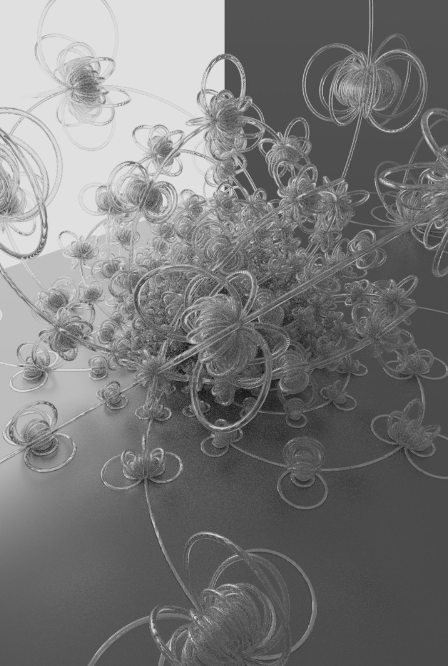
Fractal rendered with glass material, rough metallic floor, and area light in background.
2. Volumetric Path Tracing
Now that the path tracing loop has been properly ported to the GPU, implementing volumetric path tracing in an efficient way is not too hard. I based my implementation on PBR's volume integrator with homogenous media. The path tracer is capable of rendering volumes that have constant absorption and scattering coefficicients throughout their entirety. Here is an outline of a modified version of the code above that accounts for participating media:
1
2
3
4
5
6
7
8
9
10
11
12
13
14
15
16
17
18
19
20
21
22
23
24
25
26
27
28
29
30
31
32
33
34
35
36
37
38
39
40
41
42
43
44
2
3
4
5
6
7
8
9
10
11
12
13
14
15
16
17
18
19
20
21
22
23
24
25
26
27
28
29
30
31
32
33
34
35
36
37
38
39
40
41
42
43
44
fn extendPath(
    imgCoord : vec2i,
    oIn : p_vec4f,
    dIn : p_vec4f,
    bIn : p_vec4f,
    tIn : p_vec4f
    ) {
    //break input vec4fs into component parts & initialize seeds/paths
    ...

    var res : RayHit = trace(o, d);

    var bMediaInteraction = false;
    if (isInVolume(o)) {
        //sample scattering distance from absorption and scattering coefficients
        var scatteringDistance = ...;

        bMediaInteraction = scatteringDistance < res.dist;

        //update throughput
        b *= ...;

        //if the ray scattered, update the position and direction
        if (bMediaInteraction) {
            o = o + d * scatteringDistance;
            d = samplePhaseFunction(&random_seed);
        }
    }

    if (!bMediaInteraction && res.bHit) {
        //evaluate surface interaction like above
        ...
    }

    //NOTE: move Russian Roulette here to also randomly terminate scattering paths
    if (bounces > 10) {
        ...
    }

    if (!bMediaInteraction && !res.bHit) {
        //the path escaped the scene and hit the skylight
        ...
    }
}
The actual implementation of the code in lines 15-27 depends on what type of media the path tracer is rendering. In the example below, I used a volume defined only by a scattering coefficicient (i.e., no absorption). The volume had a high probability of scattering red light but a lower probability of scattering blue and green light. So, near the light source, the ball appears red, as much of the light which is scattered towards the camera is red light. However, only blue and green light can reasonably reach points further away from the light withouth scattering, so the rest of the sphere is a teal color:
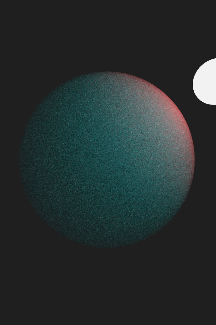
Homogenous scattering volume with different scattering probabilities for different wavelengths of light.
Based on this chapter, I modeled scattering and absorbing materials like this:
1
2
3
4
5
6
7
8
9
10
11
12
13
14
15
16
17
18
19
20
21
22
23
24
25
26
27
28
29
30
31
32
33
2
3
4
5
6
7
8
9
10
11
12
13
14
15
16
17
18
19
20
21
22
23
24
25
26
27
28
29
30
31
32
33
if (isInVolume(o)) {
    //properties of the volume
    var sigma_s : vec3f = SCATTERING_COEFFICIENT;
    var sigma_a : vec3f = ABSORPTION_COEFFICIENT;

    //the transmittance coefficient is the combination of scattering and absorption
    var sigma_t : vec3f = sigma_s + sigma_a;

    //pick a channel (i.e., R, G, or B) to importance sample
    var sampledChannel = i32(floor(rand1(&seed) * 3.));

    //importance sample exp(-sigma_t * x)
    var scatteringDistance = -log(1. - rand1(&seed)) / sigma_t[sampledChannel];
    //the nearer of the scattering distance & surface intersection distance
    var t = min(scatteringDistance, res.dist);

    //least distance == scattering distance => vertex is a media interaction
    var bMediaInteraction = t < res.dist;

    //calculate pdf of sampled distance
    var tr = exp(-sigma_t * t);
    var density = bMediaInteraction ? tr * sigma_t : tr;
    var pdf = dot(density, vec3f(1.)) * (1. / 3.);

    //update transmittance based on whether or not the path scattered
    b *= tr * (bMediaInteraction ? sigma_s : vec3f(1.)) / pdf;

    //if this is a media interaction, update position and direction
    if (bMediaInteraction) {
        o = o + d * dist;
        d = uniformSampleHemisphere(&seed);
    }
}
It begins by computing "sigma_t", which is a vector representing the probability light being scattered or absorbed over a distance. To reduce variance, it is best to importance sample the random distance the path will walk; however, with different scattering and absorption probabilities for different colors of light, importance sampling becomes more complex. First, a channel to importance sample is randomly picked (line 10). Then, the channel is importance sampled to generate a scattering distance (line 13), which is the distance the path would need to travel unimpeded before scattering. To check whether the next vertex will be a media or surface interaction, line 18 checks whether the scattering distance is less than "res.dist", the nearest surface along the ray. Lines 21-23 calculate the probability density of the sampled distance; the reasoning behind this chunk of the code can be found here. Finally, the path throughput is updated (line 26) and, if the current path vertex is a media interaction, the position is updated (line 30) and the phase function is sampled (line 31) to generate a new path direction.
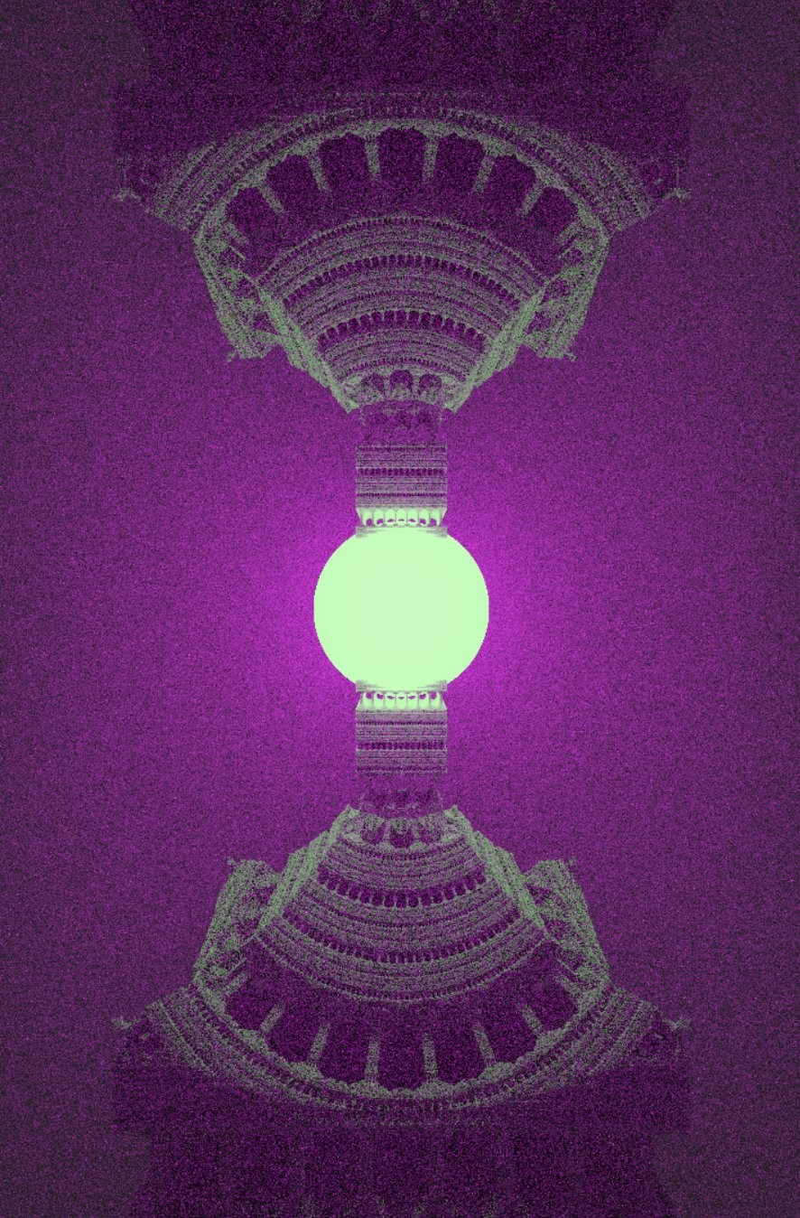
Homogenous scattering volume with different scattering probabilities for different wavelengths of light. The light is white and the fog does not absorb any wavelength of light; the color of both is due only to the scattering of the volume.
3. Wrapping Up
One of the aspects of the project that I did not write about here is procedural solid texturing. SDFs are not amenable to the usual texture or even UV-based material systems that most triangle-based renderers use. Instead, materials are evaluated as a function of world-space position (hence the term "solid texturing"). Additionally, rather than this material being precomputed, it is calculated at the time of intersection. I chose not to go into to much detail about procedural solid texturing here because I am hoping to explore more complex materials in the future.
Additionally, I will post something soon about using next event estimation in this path tracer. Typically, path tracers which work with BVH/KD-tree scenes have different, more efficient intersection functions for calculating only visibility (i.e., "any-hit" vs. "nearest-hit"); however, with ray marching, there is no difference between the two. This could allow a path tracer to treat ray traces which extend the path the same as ray traces for visibility, meaning those could "overlap" the same way that different paths can overlap by regenerating while others continue.